Your FIRE number: every major method, calculated and compared

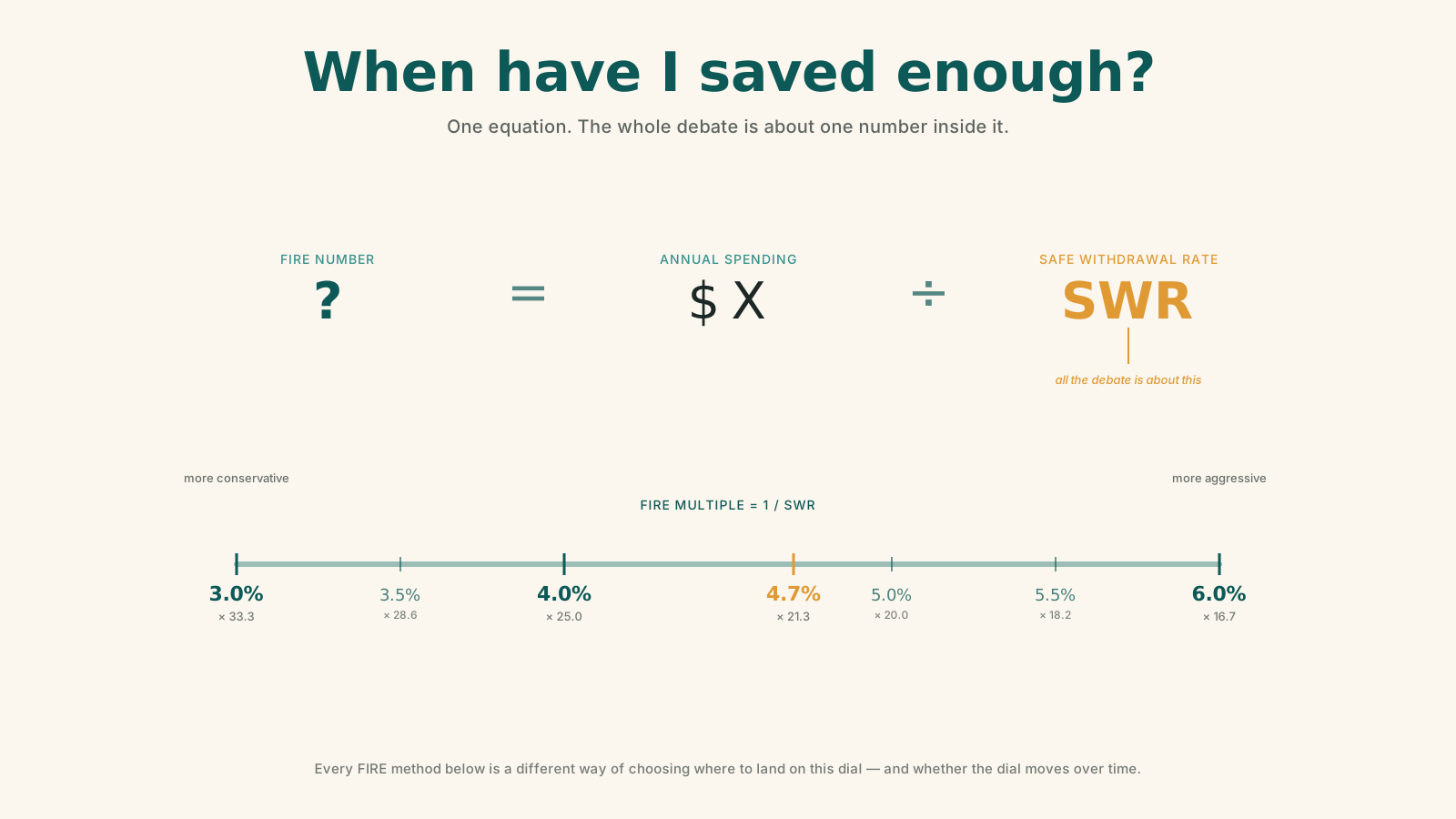
There's one question that defines the entire financial-independence movement: when have I saved enough?

Below the surface, every FIRE calculator answers it with the same equation. The whole field — the 4% rule, Monte Carlo, valuation-aware rates, dynamic guardrails, Coast and Barista variants — is a long argument about how to set one number inside that equation.

This post is the field guide. We'll start with the equation, then walk through every major method that fills it in: how each one works, what it assumes, what it gets right, where it breaks. By the end you'll know which one to use as a beginner, which one to graduate to, and how the best modern calculators stack them together. No finance degree required.

A note on what this is. Educational research, not financial advice. The same numbers can support very different decisions depending on your situation — talk to a qualified professional before making big choices about retiring or claiming Social Security.

The one equation underneath everything

Every FIRE method is a variation on a single identity:

FIRE number  =  Annual spending  ÷  Safe Withdrawal Rate (SWR)
             =  Annual spending  ×  (1 / SWR)

The famous "× 25 rule of thumb" is simply 1 / 0.04 — that's it. A 3.5% SWR implies × 28.6; a 4.7% SWR implies × 21.3; a 3.0% SWR implies × 33.3. So if you spend $50,000 a year:

Safe withdrawal rate	Multiple	FIRE number
3.0%	× 33.3	$1,665,000
3.5%	× 28.6	$1,430,000
4.0%	× 25.0	$1,250,000
4.7%	× 21.3	$1,065,000

The entire debate is about how to set the SWR and how to let it move over time. Almost every refinement below tweaks one of three knobs:

1. What rate you start at — a fixed historical floor, a forward-looking forecast, or a number tied to today's valuations.
2. Whether the rate is static or adapts — set-and-forget, rate guardrails, or fully dynamic each year.
3. What you net out first — taxes, Social Security, pensions, rental income, part-time work.

Hold that scaffold in mind. Every method below is a different answer to those three questions.

Method 1 — The 4% rule (Bengen / Trinity, and the 2025 update)

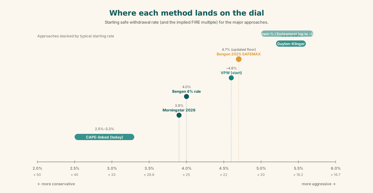
How it works. Withdraw 4% of the portfolio in year one. Each subsequent year, raise that dollar amount by inflation — ignore the portfolio value thereafter. Your FIRE number is spending × 25.

Where it came from. Bill Bengen's 1994 paper in the Journal of Financial Planning tested every 30-year rolling retirement starting in 1926 on a roughly 50/50 US stocks/intermediate-Treasury portfolio. He found the worst-case starting rate that never depleted in 30 years — about 4.15%, rounded to 4%. He called this the SAFEMAX. The Trinity Study (Cooley, Hubbard, Walz, 1998) reached a similar conclusion using a success-rate table approach.

The 2025 revision. In A Richer Retirement (Wiley, August 2025), Bengen raised SAFEMAX to 4.7% — driven not by sunnier return assumptions, but by broader diversification: adding mid-cap, small-cap, micro-cap, international equity, and T-bills to the original two assets. He frames 4.7% as a floor — the rate that survives the single worst historical start (the 1968/1966 stagflation cohort). The average SAFEMAX across all historical starts is closer to ~7.1%, and Bengen now suggests ~5.25–5.5% as a reasonable starting point for typical current retirees, pulled toward the floor by today's elevated equity valuations and inflation risk via a two-factor model.

What it assumes. A 30-year horizon, tax-advantaged accounts (no tax drag), rigid real spending (no flexibility), US historical returns, a single static allocation, and no other income sources.

Strengths. Trivially simple. One number. Battle-tested against the worst real sequences in US history. Perfect for goal-setting and explaining the concept to a beginner.

Limits.

• Built for ~30 years — too aggressive for the 40–60-year horizons typical of an early retiree.
• Ignores current valuations and yields. Every historical failure clustered at high-CAPE entry points, as today is.
• Assumes rigid spending; real retirees flex.
• US-only data, with all the survivorship-bias caveats.
• Ignores taxes and outside income.
• The inflation ratchet compounds dangerously in stagflation — two 7% inflation years lift a $100k draw to ~$114k regardless of how the portfolio is doing.

Best for: quick goal-setting, traditional ~30-year retirements, conservative temperaments, beginners learning the concept.

Method 2 — Forward-looking fixed SWR (Morningstar, 3.9% for 2026)

How it works. Mechanically the same as the 4% rule — withdraw a fixed amount, raise by inflation each year — but the starting rate is derived from forward-looking capital-market assumptions run through Monte Carlo, targeting a 90% success probability over 30 years. It's the 4% rule with an honest 2026 number plugged in.

The 2026 number. Morningstar's base case is 3.9% (up from 3.7% for 2025; 3.3% in 2021). That implies a FIRE multiple of roughly × 25.6. Their research also finds the highest fixed SWRs come from moderate equity weights (~30–50%) — because for a level-spending retiree, volatility matters more than expected return.

The critical warning. Morningstar explicitly says do not reset your spending each year to their latest number. The 3.9% is a starting-point gauge, not an annual instruction. Treat it as a temperature check on the climate at the moment you retire.

Strengths. Reflects today's valuations and bond yields rather than a century of averages — more honest when CAPE is high. Updated annually, so you always have a current benchmark.

Limits. Output is only as good as the return forecasts (and forecasts are uncertain). Still fixed-spending and 30-year by default. Still excludes taxes and outside income in the headline number.

Best for: intellectually honest goal-setting in a high-valuation environment; a defensible conservative anchor.

Method 3 — Monte Carlo simulation

How it works. Instead of one deterministic path, simulate thousands of randomized return and inflation sequences. For a candidate FIRE number and spending plan, report the probability of success — the share of runs in which the portfolio is still alive at the end of the horizon. Solve for the portfolio (or SWR) that hits a chosen success threshold, commonly 85–95%.

The deeper post: Will my money last? A beginner's guide to the Monte Carlo retirement calculator →.

What it actually does for FIRE planning.

• Naturally handles lumpy cash flows — a pension starting at 65, a kid's college at year 8, Social Security at 70, a home sale in year 12.
• Communicates uncertainty as a distribution, not a binary pass/fail.
• Lets you see the cost or benefit of small changes — work two more years, trim spending 10%, shift the stock/bond mix.

The big "but." Two limitations matter.

First, the modeling choice. Naïve Monte Carlo draws each year's return independently from a tidy distribution. Real markets aren't tidy — they have momentum, mean reversion, and fat-tailed crashes that arrive in clumps. The fix is bootstrapping: instead of inventing returns from a bell curve, draw blocks of consecutive actual historical years (returns and inflation jointly). This preserves the stock/bond/inflation co-movement that produced every real-world failure — most notoriously the 1970s.

Second, "probability of success" is a blunt metric. It counts a $1 shortfall in year 30 the same as going broke in year 10, and it says nothing about magnitude, timing, or how much you might leave unspent if things go well. A 95% success rate paired with a huge median ending balance can mean you over-saved and never enjoyed it.

Best for: the engine room of any serious calculator; modeling multi-source, multi-phase plans.

Method 4 — CAPE-based (valuation-linked) withdrawals

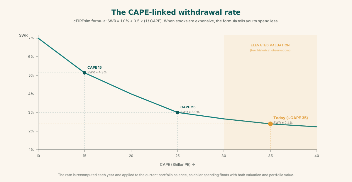
How it works. Tie the withdrawal rate to current equity valuation. Use the cyclically-adjusted earnings yield (CAEY = 1/CAPE), where CAPE is the Shiller PE — the stock price divided by the trailing 10-year average of real earnings:

Withdrawal rate  =  a  +  b × (1 / CAPE)

Common parameter sets:

• cFIREsim default: 1.0% + 0.5 × (1/CAPE)
• Early Retirement Now default: 1.75% + 0.5 × (1/CAPE)
• Some practitioners: 1.5% + 0.5 × (1/CAPE)

Worked example with cFIREsim parameters at a CAPE of 25: 1% + 0.5 × (1/25) = 1% + 2% = 3.0%. At today's elevated CAPE (mid-30s in 2026), the same formula lands roughly 2.5–3.3%. The method automatically tells you to spend less when stocks are expensive.

Because the rate is recomputed each year and applied to the current balance, your dollar withdrawal floats with both valuation and portfolio value.

Why it's intellectually appealing. It's grounded in economic reality rather than a blind historical constant. It never mathematically runs to zero (the rate is always applied to a positive balance). And it directly addresses the single biggest documented failure driver of the 4% rule: high-CAPE entry.

Limits.

• Your spending swings year to year — uncomfortable if you want a paycheck.
• CAPE's relationship to returns has drifted (structurally higher CAPE norms since the 1990s), so the chosen parameters might be miscalibrated for the current regime.
• ERN warns: there are very few historical observations of CAPE > 30, so confidence is thin in exactly today's environment.
• Harder for beginners to grasp.

Best for: valuation-aware retirees, very long horizons, and as the initial-rate setter feeding a more dynamic engine.

Method 5 — Guyton-Klinger guardrails (2006)

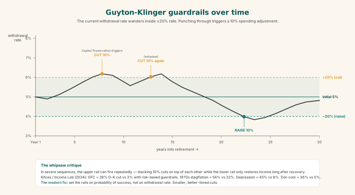
How it works. Start higher than 4% — the original paper supports 5.2–5.6% initial rates on ≥65%-equity portfolios — and govern spending with decision rules:

• Baseline: raise spending by inflation each year (a normal COLA).
• Capital Preservation Rule (ceiling): if the current withdrawal rate climbs more than 20% above the initial rate (e.g., a 5% start drifts past 6%), cut spending 10%. Suspended in the final ~15 years of the horizon.
• Prosperity Rule (floor): if the current rate falls more than 20% below initial (below 4% on a 5% start), raise spending 10%.
• Inflation rule: skip or cap the COLA after down-market years.

The big upside. Because the rails catch you, you can start materially higher than a static rule. Simple enough to run in a spreadsheet.

The well-documented failure mode — "whipsaw." In severe sequences the capital-preservation rule fires repeatedly, stacking 10% cuts on top of each other, while the prosperity rule only restores income long after recovery. A 2024 Kitces / Income Lab analysis found that a Guyton-Klinger retiree took:

• 28% income cut through the GFC (vs. 3% for a risk-based-guardrails retiree)
• 54% vs. 32% in the 1970s stagflation
• 45% vs. 8% in the Great Depression
• 36% vs. 0% in the dot-com bust

The rules are anchored to withdrawal rate, not to probability of success, so they cut too hard in some states and too little in others. Recovery can take years. This is the central critique that drove development of the risk-based guardrails described below.

Best for: flexible retirees who want a higher starting rate and a transparent, simple rule set.

Method 6 — The broader dynamic-spending family

Guyton-Klinger is one member of a family of rules that adjust spending to portfolio state. The important variants:

• Constant percentage. Withdraw a fixed % of the current balance every year. Mathematically can't deplete; income is as volatile as the portfolio. Morningstar found this and "endowment" methods support the highest starting safe rates — up to ~5.7%.
• Endowment / Yale rule. A constant-percentage variant that smooths volatility by blending prior-year spending with a target % of current balance (e.g., 70% × last year + 30% × target). Dampens swings while staying responsive.
• VPW — Variable Percentage Withdrawal (Bogleheads). Withdraw an age-rising percentage of the current balance from a lookup table — starts around 4.6% and rises with declining life expectancy, often capped to preserve a bequest. Self-adjusting; can't run dry.
• ABW — Amortization-Based Withdrawal (TPAW, ERN's CAPE tab, the economic "lifecycle model"). Each year, amortize the current portfolio over the remaining horizon at an assumed return (optionally CAPE-linked). Theoretically the most grounded — equivalent to recomputing an annuity payment annually.
• RMD method. Each year, divide the portfolio by remaining life expectancy (the IRS Required-Minimum-Distribution logic). Simple, self-adjusting, endorsed by Morningstar as a flexible option.
• Ratchet (Kitces). Only ever raises spending when the portfolio grows past a threshold; never auto-cuts. Captures upside while keeping a stable floor.
• Risk-based guardrails (Kitces / Income Lab). Set rails on probability of success — act if a fresh Monte Carlo run drops below ~80% or above ~99% — rather than on withdrawal rate. The current state-of-the-art: produces far smaller, better-timed cuts than Guyton-Klinger in historical stress tests (see the numbers in Method 5).

Family-wide trade-off. Sustainable starting rates are higher and depletion risk is essentially zero. The cost is variable income and an annual recomputation requiring discipline.

Best for: the withdrawal phase of any sophisticated plan; users with discretionary-spending flexibility.

FIRE variants — Lean, Regular, Fat, Chubby, Coast, Barista

These aren't different withdrawal methods. They're different targets and accumulation strategies layered on the same SWR math. Thresholds are community conventions, not standardized — values below reflect common US usage in 2026.

Variant	Definition	The math
Lean FIRE	Frugal full retirement, roughly < $40k/yr spend	Standard FIRE number on a low spending figure (often < $1M)
Regular FIRE	$40k–$100k/yr spend	Spending × (1/SWR)
Chubby FIRE	Between Regular and Fat — comfortable, not lavish	Same formula, mid-high spending
Fat FIRE	Luxurious, roughly > $100k/yr	Same formula, large spending → large number; often a more aggressive accumulation
Coast FIRE	Have enough invested now that, with no further contributions, compounding alone reaches your full FIRE number by traditional retirement age. You only keep working to cover current expenses.	Coast number = Full FIRE number ÷ (1 + r)^n, where r = real return and n = years to traditional retirement
Barista FIRE	Portfolio covers part of expenses; part-time work (often valued for employer healthcare) covers the rest. Portfolio may stay mostly intact.	Reduced FIRE number = (Annual expenses − part-time income) ÷ SWR. E.g. $40k expenses − $10k work = $30k → $750k at 4%

Worked example — Coast FIRE. You spend $50k/year and your full FIRE number at 4% is $1.25M. You're 35; traditional retirement is at 65 (n = 30); you assume a 5% real return. Coast number = $1,250,000 ÷ (1.05)^30 = $1,250,000 ÷ 4.32 ≈ $289,000. If you already have ~$289k invested today, compounding alone lands you at $1.25M at 65 with zero further contributions — you just need to cover your current expenses until then.

Worked example — Barista FIRE. Same $50k spend, but you'll work a part-time gig earning $20k/year. Your portfolio only needs to fund the $30k gap. At 4%, that's $30k × 25 = $750,000 — a $500k smaller target than full FIRE.

Why these variants matter so much. Coast and Barista are the two most computationally distinct from "vanilla" FIRE. Coast is a future-value problem (does today's pot compound to target without additions?). Barista is just FIRE on net expenses after earned income. Both massively shorten the timeline for younger or flexible users — and both are more sequence-risk-resilient, because earned income reduces withdrawals exactly during bad markets.

Catch. Barista assumes durable part-time work and pre-Medicare healthcare access (a major US-specific concern). Coast assumes you won't touch the money early and that real returns cooperate.

Inflation and taxes — the two adjustments most calculators get wrong

Inflation

Two design choices matter.

Real vs. nominal modeling. Run everything in real (inflation-adjusted) terms and the SWR rule is automatically purchasing-power-preserving. Or model nominal returns with an explicit inflation series. Pick one and stick to it.

Inflation as a correlated risk. The 1970s prove inflation and poor real returns arrive together. A credible engine resamples inflation jointly with returns (historical bootstrap), not a flat 2–3% assumption that ignores stagflation entirely. Bengen calls inflation the retiree's greatest enemy precisely because the COLA ratchet compounds against a falling real portfolio — two 7% inflation years lift a $100k draw to ~$114k regardless of how the markets are behaving.

Taxes

The classic Bengen / Trinity studies assumed tax-advantaged accounts and modeled no tax drag. The headline SWR is therefore pre-tax in spirit but after-tax in arithmetic — and your real-world after-tax SWR is lower.

A tax-aware calculator needs:

• Account-type buckets — taxable, traditional (pre-tax) and Roth (after-tax) — each with different treatment.
• Capital-gains vs. ordinary-income rates on withdrawals.
• Withdrawal sequencing and Roth-conversion ladders — especially the pre-59½ bridge for early retirees.
• State taxes, plus interactions with Social Security taxation and IRMAA (the Medicare premium surcharge triggered by higher income).

The practical move: convert the user's after-tax spending need into a pre-tax withdrawal requirement, then size the portfolio off the grossed-up figure. Don't pretend taxes don't exist.

Income sources — solve for the gap, not the gross

Most FIRE conversations price the portfolio as if it has to cover everything. It usually doesn't. Guaranteed and passive income — Social Security, pensions, rental NOI, a part-time job — reduces what the portfolio must do.

The core technique:

Portfolio FIRE number  =  (Annual spending  −  guaranteed/passive income)  ÷  SWR

But timing matters. Social Security at 67 or 70, a pension at 65, rental income starting now — these are lumpy, time-shifted cash flows, not a flat offset. Two rigorous handlings:

1. NPV-offset (deterministic). Compute the present value of each future income stream (use actuarial life-expectancy weighting for uncertain longevity). Subtract it from the required portfolio.
2. Cash-flow injection (simulation). Feed each stream into the Monte Carlo engine as a dated inflow. The portfolio only funds the residual in each year. Cleaner for a calculator; naturally handles "bridge" periods (retire at 50 → portfolio carries you alone until Social Security at 70).

Floor-and-upside framing

A powerful way to present the result. Cover essential spending with guaranteed income — Social Security + pension + an optional immediate annuity or TIPS ladder = a "floor." Fund discretionary spending with a more aggressive, flexible SWR.

Morningstar's 2026 research shows that delaying Social Security and leaning on guaranteed income is one of the highest-value retirement levers available — and that a long-term-care shock can pull the safe starting rate from 3.9% down to ~3.5%. Worth modeling.

Rental income is its own sub-model: net operating income (after vacancy, maintenance, management, property tax, insurance) treated as an inflation-linked stream, with the property's equity optionally counted as a terminal/liquidation asset rather than a withdrawal source.

Side-by-side comparison

Method	Starting rate (typical)	Adapts to markets?	Depletion risk	Income stability	Complexity	Best default for
4% Rule (Bengen / Trinity)	4.0% (4.7% updated floor)	No	Real on long horizons	High	Very low	Beginners, goal-setting
Forward-looking fixed (Morningstar)	3.9% (2026)	No (annual gauge)	Low at 90% target	High	Low	Conservative anchor
Monte Carlo	Solves for target	n/a (engine)	Quantified as P(success)	Depends on rule	Medium–high	The engine itself
CAPE-based	~2.5–3.3% (today)	Yes (valuation)	~Never (current-balance)	Medium	Medium	Valuation-aware, long horizons
Guyton-Klinger	5.2–5.6%	Yes (rate rails)	Low	Low (whipsaw risk)	Medium	Flexible, spreadsheet users
Dynamic (VPW / ABW / RMD / risk-rails)	4.6–5.7%	Yes	~Never	Variable	Medium–high	Sophisticated withdrawal phase
Coast / Barista	n/a (target reframing)	n/a	n/a	n/a	Low	Young / flexible accumulators

The recommended architecture for a 2026 calculator

No single method wins on all of accuracy, ease, flexibility, and realism. The right answer is a layered hybrid — a deterministic front end that gives an instant, intuitive number, and a simulation back end that supplies rigor and probability. Dynamic spending and income/tax modeling get added as you go deeper.

Layer 1 — Deterministic headline (instant). Show spending ÷ SWR immediately, with a valuation-aware default SWR rather than a blind 4%. Concretely: default the starting rate from a CAPE formula (e.g., min(4%, 1.75% + 0.5/CAPE) pulling live CAPE), or offer a slider preset to today's Morningstar 3.9% and Bengen's 4.7% as bookends. This is the number that hooks the user and sets the goal.

Layer 2 — Historical-bootstrap Monte Carlo (rigor). The engine. Block-resample actual historical years (returns and inflation jointly) rather than i.i.d. Gaussian draws. This is the single most important accuracy decision — it preserves the stock/bond/inflation co-movement that produced every real-world failure (1929, 1966, 1973). Report probability of success and the spending-magnitude/ending-balance distributions (percentile fans). Let users set the success threshold (default 90%) and horizon (default to their horizon — early retirees need 40–60, not a blanket 30).

Layer 3 — Dynamic withdrawal overlay (realism and higher rates). Let users toggle a spending rule: fixed-real (the conservative default) → risk-based guardrails (the recommended advanced default, since it beats Guyton-Klinger on cut magnitude and timing) → VPW / ABW / RMD. Surface the trade-off explicitly: "Accepting flexible spending raises your sustainable starting rate from ~3.9% to ~5.7%, but means your income varies."

Layer 4 — Income and tax engine (accuracy). Model Social Security, pensions, rental NOI, and part-time/Barista income as dated cash-flow injections into the simulation (not flat offsets), each with its own start date, COLA treatment, and taxation. Add account-type buckets (taxable / traditional / Roth) with withdrawal sequencing and a Roth-ladder option for the pre-59½ bridge. Convert after-tax spending needs to pre-tax withdrawal requirements. Implement Coast FIRE as a future-value check and Barista / variant targets as net-of-income reframings of the same engine.

Layer 5 — Honesty features. Live CAPE display with a "valuations are elevated" flag. A sequence-of-returns stress test that forces a bad first 5 years — the retirement red zone. A long-term-care shock toggle (Morningstar shows it can cut the safe rate ~0.4 percentage points). And a clear "this is not advice" framing throughout.

Defaults by user level

Beginner → the 4% rule, shown as a single number. Lead with Spending × 25. Let them see × 21 at 4.7% and × 28 at 3.5% as a conservative/aggressive toggle. It's intuitive, memorable, and motivating — exactly the right tool for goal-setting, where the job is to give a target to save toward, not to govern a live withdrawal. Pair it with one honest caveat: "real early retirements need a lower rate and more flexibility; refine below."

Intermediate → forward-looking fixed SWR + historical Monte Carlo, fixed-real spending. Default the starting rate to a valuation- or forecast-aware figure (Morningstar-style ~3.9%, or CAPE-derived). Show a probability of success from the historical-bootstrap engine over their horizon, with Social Security and pension cash flows turned on. The sweet spot of rigor and comprehensibility — it corrects the 4% rule's two biggest blind spots (long horizons, high valuations) without demanding the user manage a dynamic rule.

Advanced → full hybrid with risk-based guardrails, taxes, and multi-source income. Historical-bootstrap Monte Carlo + risk-based guardrails (probability rails, not rate rails) + the full tax / account-location / income engine + CAPE-linked initial rate + sequence and LTC stress tests. This lets a sophisticated user justify a higher starting rate (5%+), see exactly when and how much they'd need to cut, and model the real levers — Social Security timing, Roth conversions, rental income, Barista bridges — that actually move the number.

Why this ladder. Each tier adds precisely the capability the previous one lacks: the beginner needs a goal (simplicity wins), the intermediate needs probability and horizon honesty (forward-looking + Monte Carlo), and the advanced user needs adaptive spending and after-tax, multi-income realism (guardrails + tax/income engine). The same underlying simulation powers all three — you're just exposing more of it as the user climbs.

A small glossary of terms used above

• SWR (Safe Withdrawal Rate) — the percentage of the starting portfolio you can withdraw (then inflation-adjust) without depleting it over the horizon. The variable every method is trying to set.
• SAFEMAX — Bengen's worst-case historical SWR: the rate that survived the single worst starting year. A floor, not a recommendation.
• CAPE / Shiller PE — stock price ÷ trailing 10-year average of real earnings. High CAPE has historically predicted lower future returns.
• Sequence-of-returns risk — the danger that poor returns early in retirement (while you're withdrawing) permanently impair the portfolio, even if average returns are fine.
• Red zone — the ~5 years before and after retirement when a bad market does the most damage.
• COLA — the inflation raise applied to a withdrawal or income stream (e.g., Social Security's annual raise).
• Floor-and-upside — cover essential spending with guaranteed income (Social Security + pension + annuity + TIPS); fund discretionary with a flexible portfolio.
• Bootstrap (block resampling) — building Monte Carlo paths from blocks of actual consecutive historical years rather than independent random draws. Preserves real-world correlations.
• Risk-based guardrails — guardrails that trigger on probability of success rather than on withdrawal rate. The current state-of-the-art for dynamic withdrawals.
• Coast FIRE — having enough invested now that compounding alone reaches your FIRE target by traditional retirement age, with zero further contributions.
• Barista FIRE — semi-retirement where the portfolio covers part of expenses and part-time work covers the rest. FIRE number computed on net expenses.

Key takeaways

• One equation does it all. FIRE number = annual spending ÷ SWR. Every method is just a different way of choosing the SWR (and what you net out of "annual spending" first).
• × 25 isn't sacred. It's 1 ÷ 0.04. Move the rate and the multiple moves with it: × 33 at 3%, × 25 at 4%, × 21 at 4.7%.
• The 2025 Bengen update is real, but conditional. SAFEMAX rose from ~4.15% to 4.7% because of broader diversification. It's still a floor, and today's high CAPE pulls a typical retiree toward ~5.25–5.5%, not the headline.
• Forward-looking ≠ historical. Morningstar's 3.9% for 2026 is what a balanced 30-year retiree gets when today's valuations and yields are honestly priced in. Don't reset your spending to it annually — use it as a starting-point gauge.
• Bootstrapping > naïve Monte Carlo. Independent Gaussian draws understate sequence and tail risk. Block-resampling actual historical years preserves the stock/bond/inflation co-movement that broke every real-world plan.
• Sequence risk is the silent killer. A flat-average calculator is blind to it. The red zone — the 5 years either side of retirement — is where it bites hardest.
• Guyton-Klinger has a whipsaw problem. It cuts hard and clumsily in severe sequences (~28% cut through the GFC; ~54% in stagflation). Risk-based guardrails are the modern improvement.
• Variable spending earns you a higher starting rate. Static fixed-real spending caps you near 3.9%. Constant-percentage and endowment methods support up to ~5.7%. The price is income volatility.
• Always solve for the gap. Social Security, pensions, and rental income reduce what the portfolio must do. Use cash-flow injections in your simulation, not flat offsets — timing matters.
• Coast and Barista shorten the timeline dramatically. Coast = today's pot compounding into the full target untouched. Barista = FIRE on net-of-earned-income spending. Both reduce sequence risk because earned income reduces withdrawals exactly during bad markets.
• Taxes matter more than the headline rate. Convert after-tax spending into a pre-tax withdrawal requirement and size the portfolio off that.
• The best calculator is layered. A simple headline up front, a bootstrap Monte Carlo engine underneath, a dynamic-spending overlay, a multi-source income/tax layer, and honesty features. Each layer adds the capability the previous one lacks.

If you want to run your own numbers right now, open the Monte Carlo retirement calculator →. It's the Layer-1 + Layer-2 version of the architecture above: a deterministic headline plus a 10,000-run simulation engine, all in your browser. The richer guardrails and tax/income layers are on the roadmap.